Transposing data is a useful feature that allows you to switch rows and columns.

Perhaps you have a dataset that has been presented across the columns. As you add new columns of data, the presentation may become too wide.

Transposing your data can help to rearrange the data to a layout that is easier to manage by turning the columns into rows.

In this blog post, I will show you three easy methods you can use to transpose your data. Download the example workbook to follow along!

What Does It Mean to Transpose Data?

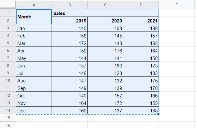
Transposing tabular data means altering the positions of rows and columns by flipping the range about its diagonal axis. Rows become columns and columns become rows.

Above you can see an example of the transpose of a range of data.

There are three popular methods of handling this operation inside Google Sheets.

1. The Paste Special method – In this method, the range is copied and pasted through the Paste Special command.
2. The TRANSPOSE function – This function takes an array as an argument and returns the transpose as output.
3. The Apps Script Method – In this method, you use the Google Apps Script to develop code that can automatically transpose the tabular array.

Now to discuss each of these three methods in detail.

Transpose Data with Paste Special

The first and most straightforward way of transposing data in Google Sheets is by using the Paste Special method.

Select the entire range you want to transpose, and press Ctrl + C on your keyboard to copy the range. In this example, the range is A1:D14.

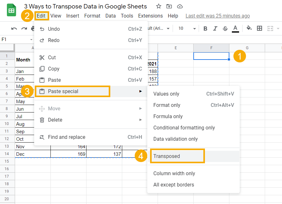
1. Select the destination cell (F1 in this case).
2. Go to the Edit menu.
3. Click on the Paste special option.
4. Click on the Transposed option to paste the copied data transposed.

You will see that the data is now transposed in cell F1 and subsequent cells. The Months are now in rows and the years of Sales are in the columns.

Transpose Data with the TRANSPOSE Function

Another way of transposing tabular data is using the TRANSPOSE function. It is an array function that operates in a way that every row is converted into a column and vice versa.

Syntax for the TRANSPOSE Function

TRANSPOSE ( array_or_range )

• array_or_range – is a mandatory argument for which the function alters the positions of rows and columns.

Example with the TRANSPOSE Function

= TRANSPOSE ( A1:D14 )

To transpose the data present in cell A1:D14, select cell F1 and insert the above formula.

You will see the transposed output spanned across the cells starting from F1.

Tips for the TRANSPOSE Function

Transpose Data with Apps Scripts

The first two methods we discussed are pretty straightforward, and they are easy to apply to transpose your data.

However, there is another way to automate the process of transposing by writing an Apps Scripts macro. You can copy the code below and paste it into your Apps Script interface to transpose the data.

If you are new to Google Apps Scripts, then check out the beginner’s guide for Apps Scripts.

function transpose() {
  
  //Defining the spreadsheet variables and setting ranges
  var ss = SpreadsheetApp.getActiveSpreadsheet();
  var sheet = ss.getActiveSheet()
  var range = sheet.getRange(1, 1, sheet.getLastRow(), sheet.getLastColumn()).getValues();

  //Defining a blank array that can hold the result
  trans = [];
  //transpose the data stored in range variable
  for(var column = 0; column < range[0].length; column++){
    trans[column] = [];
    for(var row = 0; row < range.length; row++){
      trans[column][row] = range[row][column];
    }
  }
  //printing values stored into trans variable on spreadsheet range
  sheet.getRange(1, 6, trans.length, trans[0].length).setValues(trans);

}

Explanation

• You first have to name the function. You can give any name of your choice, but it is a good practice to use the names related to your task such as transpose.
• In the first section, you define the spreadsheet variables and ranges using the SpreadsheetApp() clause over getActiveSheets() and getRange() methods respectively. the getLastRow() and getLastColumn() methods are used to get a dynamic row and column ranges. The getValues() method returns values from the selected range.
• Then, you define an empty array named trans that can hold the transposed result within.
• The first for loop starts running from column 1 of the selected range until the last column from the range. The column increment is set by 1 unit and then the results generated will be stored in a subset named column from the trans array. This for loop will take columns from the range and store them as columns in the trans array.
• Within the first loop, the second for loop runs for each row until it reaches the last row in the selected range and then returns the transposed output by altering rows and columns positions.
• Finally, we use the setValues() method after both loops end, to paste the values from the trans array into the active sheet starting from first row in sixth column (G). You can change the column positions as per your convenience but remember to not overlap the original layout.

That’s it! You now have your own script that can automate the transpose task every time you run it.

Hit the Run button to execute this script, and you can see in the sheet that data is now transposed in column G and onward.

Conclusions

In this article, you have seen three different ways of transposing data in Google Sheets.

Transposing is merely a method of arranging your data in a way that rows become columns and columns become rows.

If you want a static way that can also keep the original data formatting intact, Paste Special is the method you should go for.

If you are in need of a dynamic way of transposing data, then the TRANSPOSE function is best suited for you.

Finally, if you want to automate the entire process, Apps Script can also be used to transpose your data.

Keep in mind that the TRANSPOSE function or the Apps Script method won’t keep the original formatting when used to transpose your data!

Do you use any of these methods? Do you know another technique for transposing data? Let me know in the comments below!