Do you want to show minus signs as parentheses? This post is going to show you how to display any negative numbers inside brackets instead of with a dash!
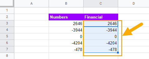
The most common way to represent a negative number has been to precede the number with a dash.
For the sake of readability in a large collection of numbers, it has become common to represent a negative number by surrounding its absolute value with parentheses.

This post explains how you can show your negative numbers inside parentheses in Google Sheets.
Show Negative Numbers in Parentheses with Financial or Accounting Format
Google Sheets has a variety of number formats that impact the display of negative numbers.
Two of the number formats explained here show negative numbers in parentheses by default, so they are a perfect choice.
One such number format is the financial format, named for its heavy use in financial performance reporting.
Follow these steps to implement the financial format,
- Select the cells containing your numbers.
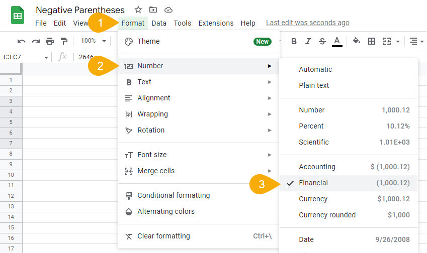
- Go to the Format menu.
- Select the Number submenu.
- Select the Financial format option.
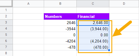
As seen above, the display of your selected numbers changes.
There are now decimal points with two-digit precision, commas separating every thousand, and negative numbers in parentheses.
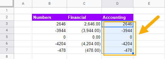
As an alternative, you could use the accounting format to show negative numbers in parentheses.
The accounting format is similar to the financial format, except that it includes a currency symbol in front and shows zero as a dash.
Follow these steps to implement the accounting format.
- Select the cells containing your numbers.
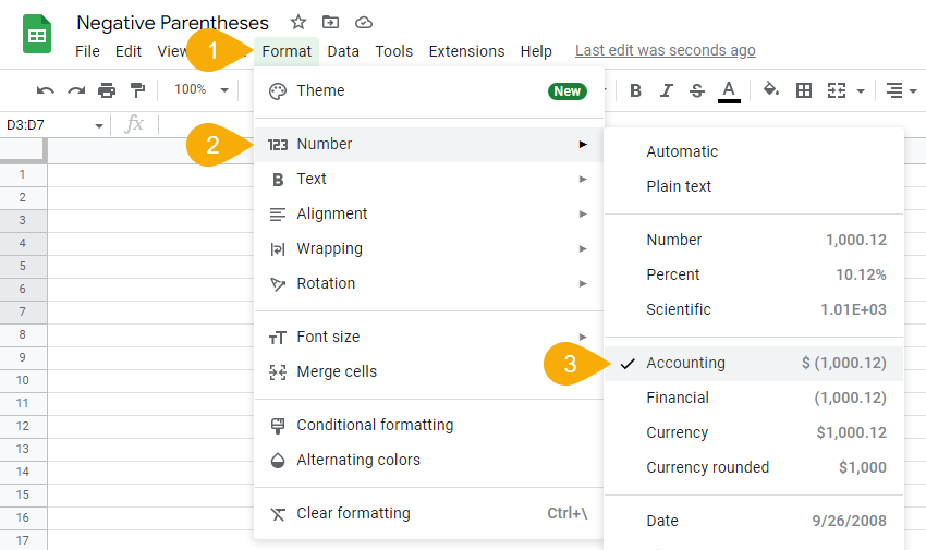
- Go to the Format menu.
- Go to the Number submenu.
- Select the Accounting number format option.
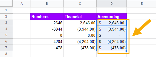
Your numbers now display in the accounting format with the parentheses around any numbers that are negative. The accounting format has the added feature that the currency symbols and decimals line up across the column.
Despite the display change, your spreadsheet calculations remain unaffected by format changes.
Show Negative Numbers in Parentheses with a Custom Number Format
Even though the financial and accounting formats provide you with the parentheses for your negative numbers, they include other format features that may not appeal to you.
If that’s the case, you may want to apply a custom number format to achieve a more ideal solution.
Follow these steps apply a custom number format with negative numbers in parentheses.
- Select your cells containing the numeric data.
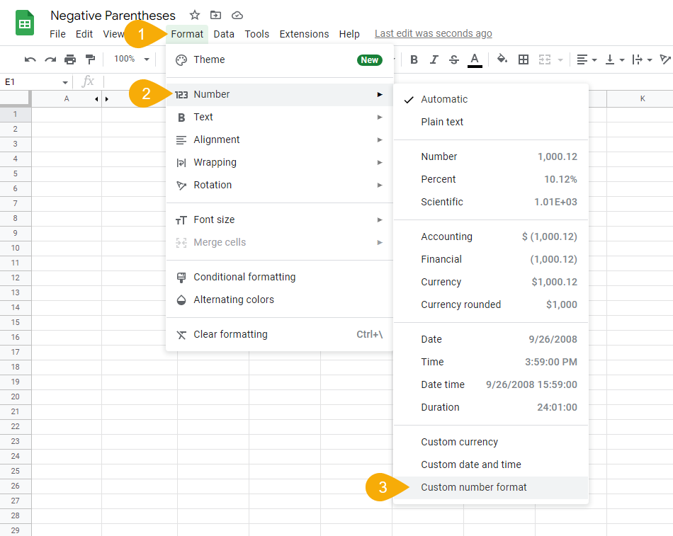
- Go to the Format menu.
- Go to the Number submenu.
- Select the Custom number format option.
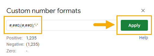
#,##0;(#,##0);"-"The Custom number formats dialog box appears.
- Paste the above custom number format into the textbox.
- Click the Apply button
This format string contains three main parts separated by a semi-colon (;) to form the custom number format.
#,##0is the desired format for positive numbers.(#,##0)is the desired format for negative number."-"is the desired format for zeros.
The above zero (0) forces at least one digit to show, rounded to the nearest integer since no decimal point is specified.
The # characters represent any additional digits that may or may not be in your cell. The comma (,) employs the use of a thousand separator.
A number like 1,000,000 exceeds the length of this string, but this string would still format that entire number.
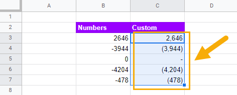
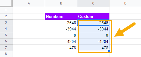
As you can see above, your custom number format now shows parentheses around negative numbers.
Show Negative Numbers in Parentheses with the TEXT Function
The TEXT function is another way to show negative numbers in parentheses. A significant effect of using TEXT is that the cell value gets converted to text, so calculations involving the cell could be impacted.
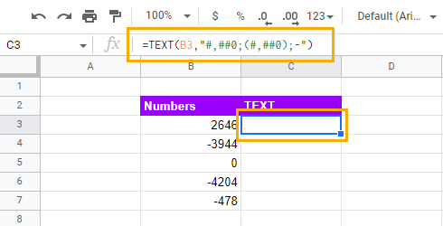
= TEXT ( B3, "#,##0;(#,##0);-" )The above screenshot shows a sample of numbers in column B. To use the TEXT function against the number in cell B3, select cell C3 and paste the above formula into the formula bar.
The first argument, B3 is simply the cell reference to the number.
The second argument is the format string, which is similar to that described in the Custom Number Format section of this post.
You must surround the format string with quotes marks ("). Any additional quotes marks (") beyond that may give you an error.

Press Enter to execute the formula, then copy the formula down to cell C7. Note that cells C4, C6 and C7 show the negative numbers in parentheses, as desired.
Show Negative Numbers in Parentheses with the QUERY Function
The QUERY function allows you to apply an operation to multiple cells at once.
Its query language includes a format feature that you can use to format your numeric results and show negative numbers within parentheses.
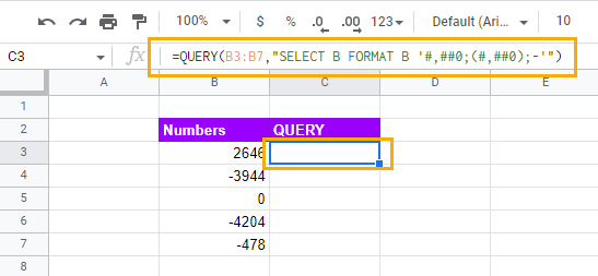
= QUERY ( B3:B7, "SELECT B FORMAT B '#,##0;(#,##0);-'" )Given a column of numbers, such as column B above, you can format the numbers into column C with one QUERY function. Select cell C3 and paste the above formula into your formula bar.
The first argument, B3:B7 refers to the data being queried.
The second argument, surrounded by double quotes ("), is the query language known as Google Visualization API language.
The SELECT B portion indicates that column B is being returned without any mathematical calculations.
The FORMAT B portion indicates that a format is being applied to column B, followed by the format detail surrounded by apostrophes (').
The format detail follows the same rules as described in the Custom Number Format section of this post.
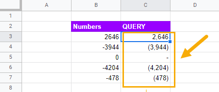
Press Enter to execute the QUERY function and you will see how all of your relevant cells in column C get automatically populated with your desired format!
Conclusions
You have several options when needing to implement parentheses for negative numbers.
If you only need a consistent display of your numbers, the financial or accounting format is a simple way to achieve parentheses around your negative numbers.
You can tweak the default behavior of the financial or accounting format by using the custom number format options.
The TEXT function can also be used to show minuses inside parentheses. This is a great option when you need to combine text with formatted numbers.
In the most complex of situations, the QUERY function offers formatting in combination with the ability to perform calculations or summarize your dataset.
Do you format your negative values in parentheses? Do you know any other ways to do this? Let me know in the comments below!


0 Comments