This post will show you all the different ways you can insert checkmarks or tickmarks into your Google Sheets.
When you use spreadsheets, you often only think of numbers and data analysis.
But the spreadsheet isn’t all just about numbers. There’s much more!
Spreadsheets have a varied range of applications because they support the use of various characters, symbols, images, and graphics.
Spreadsheets are a very dynamic tool that can be used in many different situations.
Imagine you have a project to accomplish within a specific timeline. There’d be tasks that need assigning to different people and you will also want to keep track of the progress of each task. A spreadsheet can help you do this.
These can help to add great visual indicators for at-a-glance information.
The checkmark or tickmark symbol ✔ is one of the many characters that can help make your spreadsheet a dynamic and visually interesting tool.
This post will explore all the different ways you can insert checkmarks into your Google Sheets. Get your copy of the example workbook and follow along.
Insert a Checkmark with Copy and Paste
✓✔☑✅This first method is simple and easy to use. All you need to do is copy any of these checkmark characters and paste them into your spreadsheet.
You’re not limited to these 4. You can find a variety of checkmarks with a Google search and try to copy and paste those results as well.
Insert a Checkmark with the UNICHAR Function
This method requires that you use one of the inbuilt functions called UNICHAR.
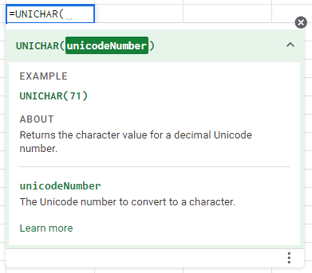
= UNICHAR ( unicodeNumber )It’s a simple function because it takes just one argument. The unicodeNumber refers to the unique number that represents the character you want the UNICHAR function to return.
Every character supported in the spreadsheet is coded using unique numbers/codes. The UNICHAR function is a text function that will help you return any character based on this unique code of the character.
Checkmarks in Google Sheets have the following unicode numbers.
9745, 9989, 10003, 10004
You can use them in the UNICHAR function as illustrated below

= UNICHAR ( 9745 )For example, the above formula will produce the ☑ character.
Take note of the preview at the top of the syntax. It will show you a preview of formula results, so you can see the character your number represents before you hit Enter.
As the unicodeNumber changes, the character in the preview also changes.

Quick Tip: If you don’t know the unicodeNumber of a character, you can use the UNICODE function to return the unicodeNumber.

= UNICODE ( text )UNICODE is another simple function with one argument. It takes a text character and returns the corresponding unicodeNumber of the character.
= UNICODE ( "☑" )For example, the above formula will give a result of 9745.
Once you have this in your sheet, you can convert the formula to a value in several ways.
Insert a Checkmark with the Emoji Keyboard
You can use checkmarks with the emoji keyboard in your spreadsheet.
The process requires a keyboard shortcut to access the emoji keyboard on your Windows device. Press the Windows key + . to open the emoji keyboard.
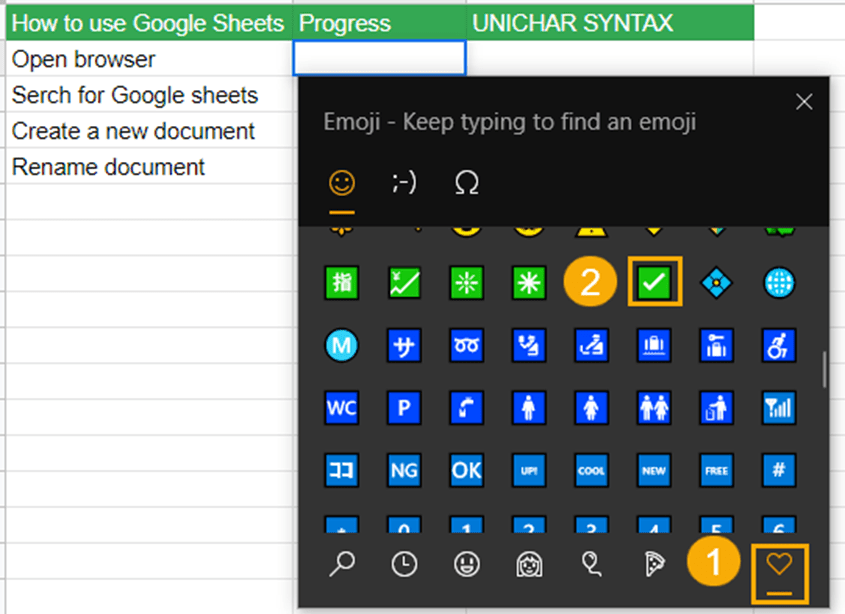

The first step to take when you want to use the emoji checkmark in your spreadsheet is to make sure you select where you want to insert the checkmark.
Then, double-click on the cell or press F2 so it’s in edit mode.
You can now use the Windows + . keyboard shortcut to open the emoji keyboard.
The emoji dialogue box will appear and you can find checkmarks emoji in the symbols collection. It is indicated by the heart icon.
Another option is to type the word check to search all the available emoji’s.
Insert a Checkmark with the IF Function
A handy way to use these checkmark characters and avoid monotony or repetition is to use them in an IF function.

A new column has been added to the workbook. The Progress column indicates tasks that are complete or incomplete.
The IF function allows you to test a logical statement. You can then specify what value to return when the logical statement is true, and a different value for when the logical statement is false.
You can test the value in the Progress column using the IF function and then return a checkmark when the task status is changed to complete.

= IF ( B2 = "completed", "✔", "-" )Select an adjacent empty cell and insert the IF formula above.
When you copy and paste this syntax, you can use the fill handle at the bottom right-hand corner of the cell to drag down and copy the formula to the other cells.
This IF formula will then insert the checkmark based on the value in the Progress column.

= IF ( B2 = "completed", UNICHAR ( 9989 ), "-" )You could also use the UNICHAR function has inside the IF statement to generate the checkmark character.
Now you can easily insert checkmarks in your cells with little effort. When you add a new set of tasks to the list, you simply need to drag down the fill handle to insert the checkmarks.
Insert a Checkmark with a Checkbox
You can insert a checkmark by using the Tick box feature in Google sheets.
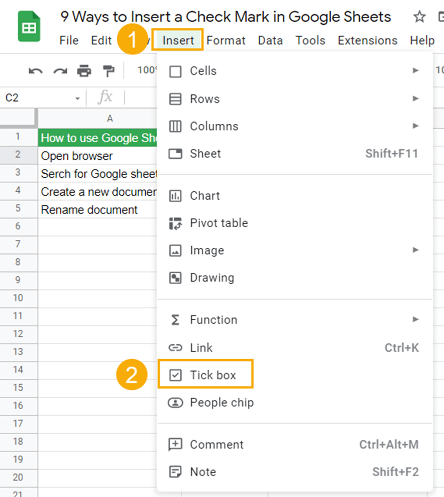
Before inserting the Checkbox, you should first select the cell where you want the checkbox to appear. Then follow these steps to insert the Checkbox.
- Go to the Insert menu option
- Select the Tick box option. With certain region settings enabled, it might also be labeled as Checkbox.

You can drag down the fill handle to copy the checkbox to the other empty cells.

To make the checkmark appear, click the space inside the checkbox.
The checkbox is a very dynamic tool that can do a lot more! You can customize some of its features.


If you look at the formula bar, you will see the value changes as you click on the checkbox.
By default, these values are set to display either TRUE or FALSE. You can change this displayed value to show something more appropriate for your situation.
For example, you might use a checkbox to create a yes or no column in your data.
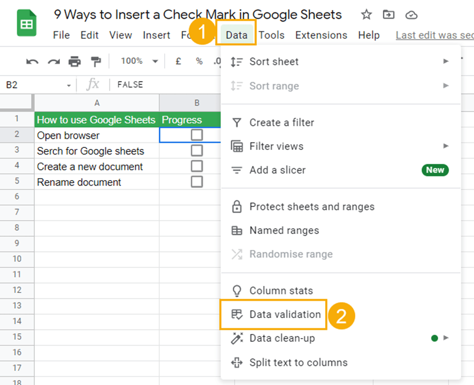
Follow these steps to change the values of the checkboxes.
- Go to the Data menu.
- Select Data Validation from the options.

- Use the Cell range option to select the cell ranges where you want to effect the change. This option can also be used to insert a Checkbox.
- The Use custom cell values box is unchecked by default. To reveal the Ticked and Unticked editor box, you have to check the Use custom cell values box.
- Use the editor windows for the Ticked and Unticked options to specify values to display when the checkbox is ticked and when it’s not ticked.
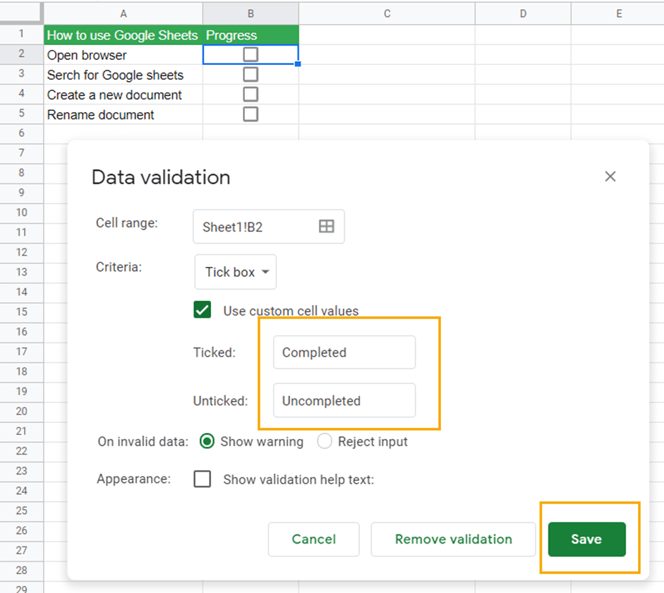
- Press the Save when you’re done.

The checkbox reflects the changes made. If you tick the box, the value in the formula bar will display Completed.
With the Checkbox, you can easily add checkmarks to a range of cells. And with a single click, you can deliver progress reports on your tasks. No codes, no functions, no formulas needed!

If you find the color of the tick box a little dull, you can change it with the Text color menu from the toolbar.
Checkboxes are a great way to make your workbook user-friendly. Check out these interesting ways in which checkboxes can be used.
- Add strikethrough format with a checkbox.
- Delete rows with a checkbox.
- Show or hide gridlines with a checkbox,
- Hide rows with a checkbox.
- How to Count Checkboxes.
Insert a Checkmark Using an Apps Script
Instead of using a checkbox, you can use an apps script to insert checkmarks to adjacent cells when certain conditions are met.
Open the Apps Script editor. Go to the Extensions menu and select Apps Script from the options.
Then copy and paste this code into your app script editor window. Make sure you click on Save and Run afterward.
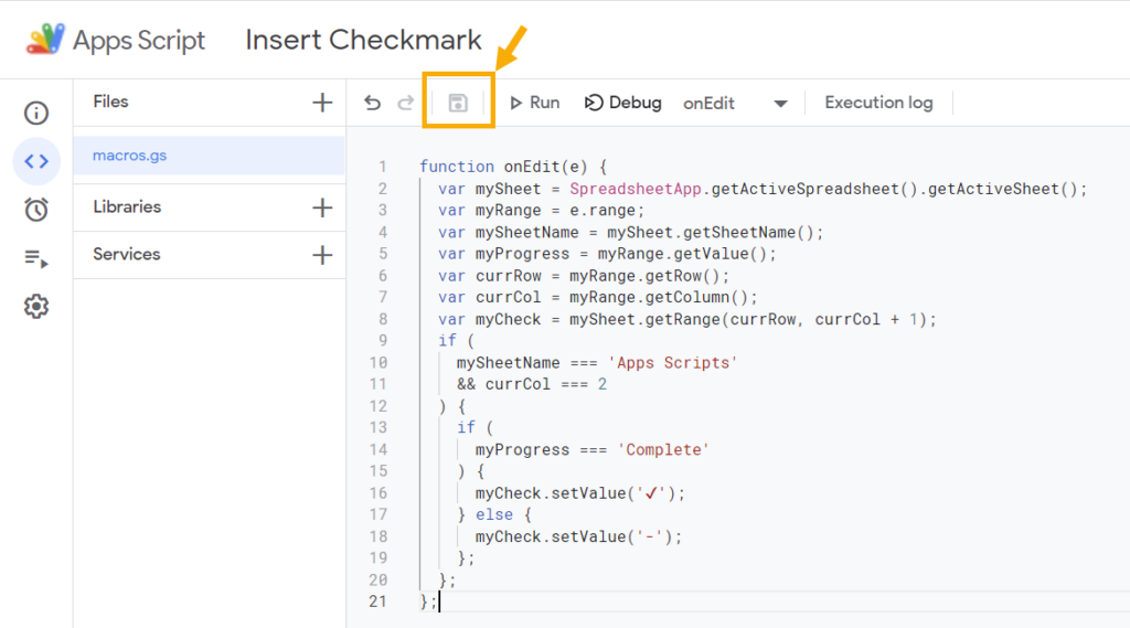
function onEdit(e) {
  var mySheet = SpreadsheetApp.getActiveSpreadsheet().getActiveSheet();
  var myRange = e.range;
  var mySheetName = mySheet.getSheetName();
  var myProgress = myRange.getValue();
  var currRow = myRange.getRow();
  var currCol = myRange.getColumn();
  var myCheck = mySheet.getRange(currRow, currCol + 1);
  if (
    mySheetName === 'Apps Scripts'
    && currCol === 2
  ) {
    if (
      myProgress === 'Complete'
    ) {
      myCheck.setValue('✔');
    } else {
      myCheck.setValue('-');
    };
  };
};
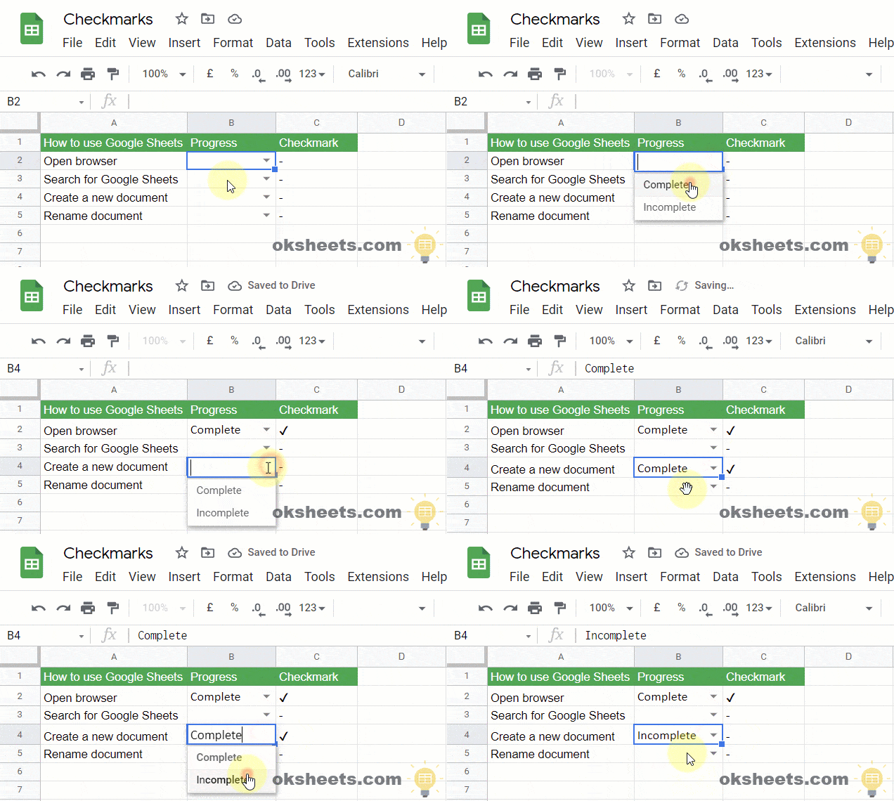
For this example, we’re keeping the same data setup used in the Checkbox method.
With the apps script, you only need to type the status of the project and the checkmark will be inserted into the adjacent cell.
This is possible because of the onEdit trigger used in the Apps Script. Every time the spreadsheet notices a change in the cell, it checks to see if the value entered inside the cell is Completed.
The IF statement in the script is responsible for testing if the progress is Complete.
If the value in the cell is changed to Completed, a checkmark will be inserted inside the adjacent cell. If not, a dash will be inserted.
Insert a Checkmark Image Inside a Cell
You can bring images from external locations into cells in the spreadsheet.
To insert a checkmark image inside a cell, follow these steps.
- Select the cell where you want to insert the image.
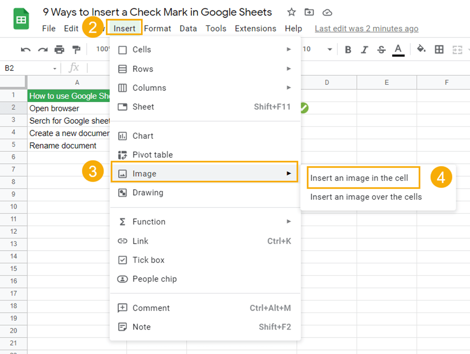
- Click on Insert from the menu.
- Select Image from the options.
- Select Insert an image in the cell from the submenu options.
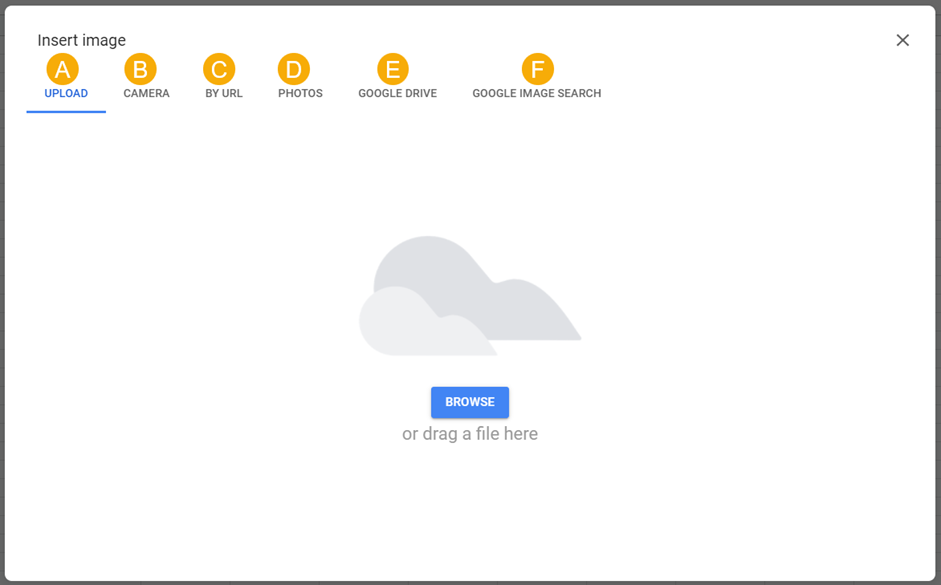
- A: UPLOAD Allows you to choose from files on your computer storage.
- B: CAMERA Allows you to take a picture of an object you want to import.
- C: BY URL – Allows you to provide the URL of the location where the image is stored and Google sheets will import it into your cell.
- D: PHOTOS Allows you to connect to your Google photos profile and import images. Use this option if the image you want to import is in your Google photos folder.
- E: GOOGLE DRIVE – Allows you to connect to your Google Drive storage to import an image.
- F: GOOGLE IMAGE SEARCH Allows you to perform a Google search for the image you want to import.

Using the GOOGLE IMAGE SEARCH option you can search for checkmark with the search bar and then choose an image from the results.
Click on the image to select it and then press the INSERT button to add the image to your sheet.

The selected checkmark has been imported into the cell.
You can also drag the fill handle down to copy it to the remaining cells.
Check out these other ways you can insert images in your Google Sheets.
Insert a Checkmark Image with the IMAGE Function
The IMAGE function is another way to insert an image into Google Sheets.
The IMAGE function is used to import images from a URL. It works just like when you use the URL option from the Insert image method.

= IMAGE ( URL, [mode], [height], [width] )- URL – Is a required argument. It is the URL link or web address of where the image is located. The URL must be entered in quotation marks.
- mode – This argument is used to provide size specifications of the image being imported. The mode argument takes only numeric values between 1 and 4. Each number in this range has been designated to carry out specific size fittings.
- 1: Resizes the image so it can fit inside the cell, It also keeps the aspect ratio to prevent distortion of the image.
- 2: Resizes the image to fill the entire cell. It doesn’t maintain the original aspect ratio.
- 3: Keeps the original size of the image.
- 4: Allows you to provide custom size settings for the imported image using the height and width argument.
- height – Allows you to specify height dimensions in pixels for the image.
- width – Allows you specify width dimensions in pixels for the image.
To use the height and width argument, you must enter 4 in the mode argument.

= IMAGE ( "https://www.oksheets.com/wp-content/uploads/2021/09/Checkmark-Image.png" )To import a checkmark using the IMAGE function, copy and paste the above formula. The result is an image hosted on this site!
Insert a Checkmark with Drawings
Creating a checkmark drawing is a method you can use to insert checkmarks in your spreadsheet.
These objects will float above the grid and are not inside a cell. They can be freely moved around the top layer of your sheet.

To create a Drawing, click on the Insert option from the menu bar and select Drawing.

You should get the Drawings dialogue box. It has a Canvas where you draw an object and Menu options for modifying your object.
Drawings provide three options for inserting checkmarks into your spreadsheet. You can use Shapes, WordArt, or the Scribble option.
Insert a Checkmark with Shapes
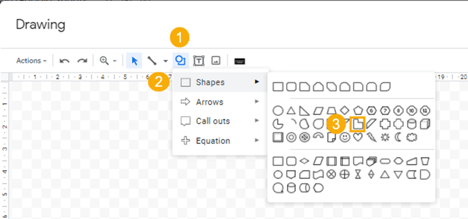
To use a checkmark using the L shape, follow these steps.
- Click on the shape icon.
- Click on Shapes.
- Select the L shape from the list of shapes.

Click and drag inside the canvas to create your shape L shape.
Make sure to rotate the L shape so it looks like a checkmark! Click and drag the rotation handle to rotate the L shape to your preferred orientation.

You can add colors and remove borders using the Fill color and Border color menu.
You must keep the image selected before you can access these menus. When you’re done, click on Save and close and the image will be imported into your spreadsheet.

The image will not fit into a cell and will float independently across the spreadsheet.
You can use the little square boxes on the edges of the image to resize it. To access more options for modifying the image, click on the three dots at the top righthand corner of the image.

Resize the checkmark drawing to fit on top of the cell you want it to appear.
Insert a Checkmark with Word Art

To create a checkmark from the Word art option found in the Drawing dialogue box follow these steps.
- Select Actions in the menu.
- Select Word art from the menu list.

After selecting the Word art option, you will get an editor window. Inside it, copy and paste a checkmark image. PRess Enter on your keyboard when you’ve added a check character.

As with the drawing of the L shape, you can add fill and border color to the image. Click on Save and close when you’re done.

You can resize it and place it on the cell you want it to appear.
Insert Checkmark with Scribble
Scribble is a feature that allows you to draw freehand sketches of objects on the canvas.
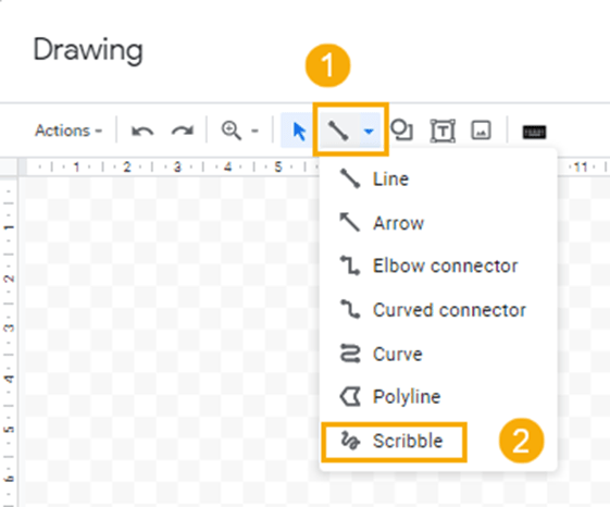
To create a checkmark with scribble, follow these steps.
- Select the Line menu.
- Select Scribble from the options.

Draw your checkmark on the canvas. Click on Save and close to insert the scribbled checkmark on your spreadsheet.

The scribbled checkmark can also be resized to fit on a cell.
Conclusions
Your situations will dictate what checkmark inserting method you should use.
For instance, if you need a checkmark for design purpose, creating a Drawing or importing a checkmark image might be the best option.
But when creating a to-do list, options like copy and paste, the UNICHAR function, emoji’s, and the Checkbox methods will be a better fit.
In the end, you may only need one or two of these methods. But it is worth knowing other options exist!
Do you use any of these ways to insert checkmarks in your Google Sheets? Let me know in the comments below!


0 Comments