This post will show you how you can extract a URL from a hyperlink in Google Sheets.
There are a few reasons why you might want to extract a URL from a hyperlink.
It could be that you may want to use the URL in another sheet or use it in an entirely different application.
Another situation where you might find yourself needing to extract a URL from a hyperlink will occur when you copy and paste data from the web.
When this happens, only the anchor text appears in your spreadsheet. You will need to do some extra work if you want to see the URL.
In this post, you will see 3 methods you can use to get the URL from a hyperlink in Google Sheets. Get your copy of the example workbook to follow along!
Extract the URL from a Hyperlink by Hover and Copy
Check out this post if you’re unsure what a hyperlink is or how to insert a hyperlink in Google Sheets. Various methods of inserting hyperlinks were explored.

This is a list of hyperlinks to other articles on this website that were copied and pasted directly into the spreadsheet. You can extract their URLs using the hover and copy method.

A quick view box containing the URL of the hyperlink shows up every time you move your mouse over a cell with a hyperlink.
Inside the quick view box, to the right of the URL, there are three other icons, each one performing separate tasks.
By hovering your mouse across them, you will see the function each one performs.

To extract the URL from the hyperlink, click on the Copy link icon.

After clicking on the Copy link icon, the URL of the hyperlink is copied to your clipboard.
This allows you to paste the copied URL into any cell you wish. You can use the keyboard shortcut, Ctrl + V, or right-click and choose Paste from the option in the menu.
In those simple and easy steps, you have extracted the URL from a hyperlink.
Extract the URL from a Hyperlink by Edit and Copy
There are 3 ways by which you can access the Edit command for a hyperlink.

The first is from the quick view box. Click on the Edit link icon.

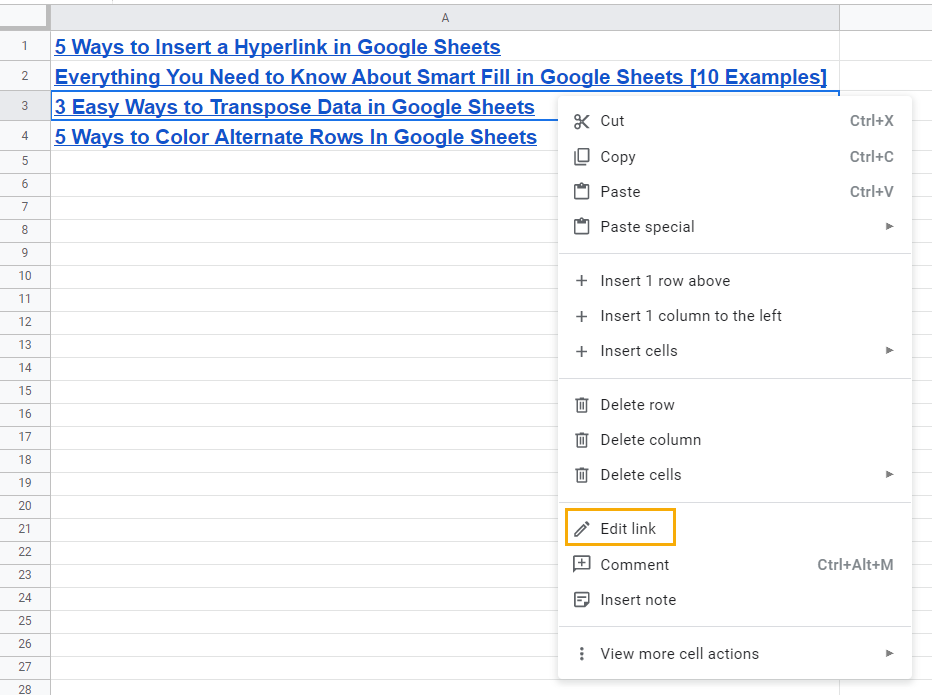
You can right-click on the cell containing the hyperlink and select the Edit link option from the menu.

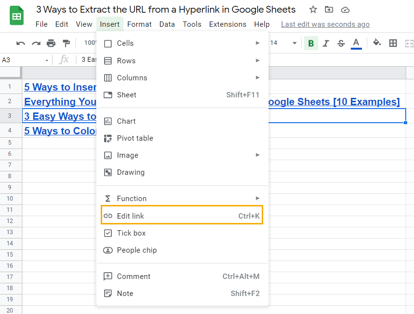
You can also access the Edit link option from the Insert menu. Also, the keyboard shortcut Ctrl + K can be used to edit the hyperlink.

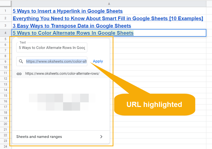
Using any one of these Edit link options will open the dialogue box you get when you want to add a hyperlink to a cell.
However, because the cell already contains a hyperlink, the Edit link command opens the dialogue box and automatically highlights the existing URL.
From this point, you can either change the URL by inserting a new one or extract the URL by simply copying the highlighted link using the keyboard shortcut Ctrl + C, or by right-clicking on the highlighted link and selecting the copy option.

After you’ve done this, click on the cell where you want to insert the URL and paste the copied link using any of the pasting methods identified earlier.
While using either one of these methods to extract URLs from hyperlinks is simple and easy to use, unfortunately, they have some limitations.
- These methods don’t allow for the extraction of URLs when the hyperlinks are contained in a single cell.

Hovering your mouse over the cell wouldn’t bring the quick view box.

And using any of the Edit link options wouldn’t reveal the URL for you to extract since there are multiple URLs in the cell.
To use these copy and paste methods to extract URLs, the hyperlinks must be contained in separate cells.
- These methods are not dynamic. They cannot be efficient for use on large sets of hyperlinked. Imagine you have hundreds of cells with hyperlinks whose URL you need to extract. It would be tedious and consume a lot of time to extract each URL. For large scale URL extraction operations, you may favour a more technical method such as using an Apps Scripts to extract the URL from a hyperlink.
Extract URL from a Hyperlink with a Custom Apps Scripts Function
There are hundreds of built-in functions in Google sheets that allow you to perform almost all kinds of operations on your data.
These functions are very efficient at producing results in a fraction of the time it will have taken you to manually perform each operation.
Unfortunately, there is no built-in function for extracting a URL from a hyperlink.
Apps Script is a feature provided by Google to enable users to create custom functions. It is based on JavaScript, and it doesn’t require any software installation or special setup on your computer.
Only a Google account and a web browser are required to access the script editor.
Check out the full guide to getting started with Apps Scripts for more details.

You can access the Script editor from the spreadsheet by going to the Extensions menu option and clicking on Apps Script.

This will open a new window in your browser that displays the google App Script editor.
In the Script editor window, you can change the name of your project from the default Untitled project by double-clicking on it.
The program controls area contains commands that allow you to perform regular editing activities on your code. You’d mostly perform the save (looks like a diskette icon), run, undo, redo, and debug operations on your code.
The files area is where your newly created codes are saved.
With Apps Script, you can create a customized dynamic function that will help you to extract URLs from hyperlinks.

Copy the code below into the code window to create and use the GetURL function.
function GetURL(input) {
  var myFormula = SpreadsheetApp.getActiveRange().getFormula();
  var myAddress = myFormula.replace('=GetURL(','').replace(')','');
  var myRange = SpreadsheetApp.getActiveSheet().getRange(myAddress);
  return myRange.getRichTextValue().getLinkUrl();
 };
After copying and pasting the script, ensure you save it so that you can use it on your spreadsheet.
When you the code on Apps Script for the first time, you will be prompted to authorize the code.
Click on Allow when prompted. When you’re done with this process, your custom Apps Scripts function will be available for use on your spreadsheet.

=GetURL(A1)You can now use the above custom function to extract the URL from a hyperlink in cell A1.
⚠️ Warning: The code and function are case sensitive, so make sure you use the exact function name used in the code!
Conclusions
While there is no built-in function to extract URLs from hyperlinks, there are a few workarounds.
You can copy URLs from the quick view box or the Edit command and paste them into a cell, but this can be tedious for large datasets.
The most efficient option would be to use a custom function. You can create a custom Apps Scripts function you can then use in your spreadsheet to extract the URL from any hyperlink.
Have you used any of these options? Are there any other methods you know of? Let me know in the comments below!


Hi there – I tried the third method “Extract URL from a Hyperlink with a Custom Apps Scripts Function”, but get an error when I tried it first in a Google sheet. Script created and Google sheet all created/being edited using same Google account.
I entered formula =getURL(A79) and pressed Return. In the cell it briefly said ‘Loading’ but then return the following error:
Error
Exception: Range not found (line 4).
Any suggestions?
The function name is case sensitive, so it has to be
=GetURL()and not=getURL().any way to rewrite this function so it can get the url from a different sheet in the same workbook? For example =GetURL(‘Sheet 2’!A1)
I just tested this situation and it works for me. Make sure the function name is an exact match to what is in the code as it’s parsed in the code as text.
I’m getting the below error when i run the script
Error
Exception: Range not found
GetURL @ Code.gs:4
TypeError: Cannot read property ‘getFormula’ of null
GetURL @ Code.gs:2
I run the script is it what I suppose to do?
nvm it works
The script is run by using it as a function in the sheet.
I get this error on the sheet,
“TypeError: Cannot read property ‘getLinkUrl’ of null (line 5).”
Remember, it’s case sensitive!
Is the function getLinkUrl or GetURL?
The formula in the Sheet “= GetURL(A3)”
Project Name: Extract URL
function GetURL(input) {
var myFormula = SpreadsheetApp.getActiveRange().getFormula();
var myAddress = myFormula.replace(‘=GetURL(‘,”).replace(‘)’,”);
var myRange = SpreadsheetApp.getActiveSheet().getRange(myAddress);
return myRange.getRichTextValue().getLinkUrl()
}
Try deleting the code and pasting it again from the post. You can also try the example workbook, as it’s working in there! Best of luck!
Does the URL have a pound sign (#) in it? I got this same error when that was the case, but not with any URL that did not have # character
Hovering over the formula on the sheets shows “Unknown function:’GetURL'”
Make sure to save the script and then refresh the workbook.
Well same here, refresh not working
Try saving and running the script at the APP Script page. When running for the first time, Google will ask for your permission run the script with your account. Accept it and then refresh the spreadsheet. Hope it works this time.
Same. I run it and the cell displays “Loading” then returns a blank cell. When I run it in Apps Script I shows the error:
Exception: Range not found
GetURL @ Code.gs:4
Is there a way to to this with hyperlinks that are also images?
I currently have colum full of formulas such as: =HYPERLINK(“https://i.imgur.com/4v5nEV6.png”, IMAGE(“https://i.imgur.com/4v5nEV6.png”)) in my file. I’d like a new column that extracts to the link itself as a value.
Currently, I am getting #ERROR! TypeError: Cannot read property ‘getLinkURL’ of null (Line 5)
Thank you so much for creating these helpful guides in advance.
In this case, I would use the FORMULATEXT function to convert the formula to text. Then you can use the SPLIT function to get the URL.
Haha, you just implied a 4th (and simplest) way to extract the URL from a HYPERLINK formula, a formula in cell A2 that fills A2 with the URL from a HYPERLINK in cell A1:
A1:
=HYPERLINK("https://www.oksheets.com/", "This Page")A2:
=INDEX(SPLIT(FORMULATEXT(A1), """"), 0, 2)First FORMULATEXT gets the full HYPERLINK formula string from A1. Then SPLIT gets the 2-5 substrings that the URL’s pair of quotes ( each
"doubled to""to escape them, then enclosed in direct quotes for the formula literal string delimiters) characters and the link_label argument (if any) pair of quotes characters separates the formula string into: [=HYPERLINK(], [] [, ], [], [)]. Finally INDEX gets the second substring, the .It doesn’t require any AppScript and so it’s flexible for different uses or combinations with other formulas.
Yes, this is a great option!
The app script would need to be used only when the link wasn’t created with a function.
Thanks Man, you save my life 👍
The code is missing a semicolon on the last line. I added it and fixed all the errors I was getting.
Thanks!
Thanks for the post John – very useful!
I encountered some errors with the range too – not sure why.
Another issue is that if you want to wrap this code in another function – eg. “IF(ISBLANK(A2),””, GetURL(A2))” it will break as it parses its own formula text to get the address. I guess there’s a cleaner way to do so but oh well.. it works now. Thanks again!
Yes, the only way to get the range address of the inputs from a custom function is to parse the formula text.
I recently updated the code for this use case on embedding the function within a function.
Is there a way to do a range? I.e. B2-B300?
Yes, but you would have to modify the code to loop through the range and extract the URL from each cell.
Or copy and paste the formula down the column.
I created the script, paid attention to the exact usage of upper/lowercase.
It says “Loading…” and then nothing, just blanks. Any suggestion?
Are you nesting functions? The script relies on parsing text and that will break it.