If you are frequently working on Google Sheets, you might have observed a dataset with first and last names being stored in two different columns.

Keeping these two fields in separate columns makes it easier for analysts to filter people based on their first or last names. This means there are more ways to explore, analyze, and summarize the data.

However, there might come situations where you need to combine the first name and last name.

For example, the HR department wants you to give the full employee name to distribute the yearly bonus, or you might want the full name to print on their official ID card.

You can identify many more scenarios where there is a need to combine the first and last names.

Inside this article, I will show 6 ways different ways of combining first and last names inside Google Sheets.

Get your copy of the example workbook and follow along with me!

The Database

This post will use a small dataset for this task with five entries.

Five people have their first and last names stored inside two different columns, as shown above. I will show you how to combine these names inside column C.

If you instead need to separate out a first and last name, then check out this post on how to split cells into multiple columns.

Combine First and Last Names Using the Ampersand Operator

The thing that most people love about Google Sheets is the availability of various simple-to-use operators.

One such operator is the ampersand (&). This operator is specifically used to combine two or more cells, irrespective of their data types.

You can use the ampersand operator (&) to combine the list of first and last names inside column C of the spreadsheet.

= A2 & B2

To combine the first and last name columns using the ampersand, use the above formula inside cell C2 and hit the Enter button to insert it.

There are various ways of applying this formula on all other rows of column C.

• You can either click and drag the formula down across C2:C6 using the small square in the lower right corner.
• You can select the range C2:C6 and hit Enter to apply the formula in C2 to all rows.
• You can copy the formula and paste it in every cell.

Here, one thing that looks incorrect is the absence of space or any other delimiter between first and last names.

The ampersand operator combines anything that is on either side of it. The operator doesn’t include any default delimiter such as a space character between the items it is joining. You have to specify it separately.

= A2 & " " & B2

Use multiple ampersands to add a space between the first and last name inside column C as shown in the formula above.

Pro Tip: You can also use another delimiter to separate the first and last names inside column C. Make sure to add it within the double quotes between two cells. For example, you could use a comma instead of a space.

The advantage of using the ampersand operator over any other function is its simplicity. You just use the & operator between any items you want to combine together.

You have the liberty to use any delimiter to separate the combined output. You can separate values using commas, spaces, semicolons, etc.

This is perfect when joining two or three items together, but it will quickly become tedious when combining anything more.

Combine First and Last Name Using the CONCAT Function

Another function that is built explicitly for the current task of combining names, is the CONCAT function. The function takes two values as an argument and combines them together.

Syntax for CONCAT Function

CONCAT ( value1, value2 )

• value1 – is a required argument that specifies either a cell reference with value or the value itself.
• value2 – is a required argument and consists of cell reference or value that gets combined with value1.

Combine First and Last Name Example

= CONCAT ( A2, B2 )

To use this function to combine the first and last names insert the above formula into cell C2.

The first argument you put is cell A2, where the first name is stored. The second argument is B2 that consists of the last name.

You will see the output as shown above.

To apply this formula across all cells where the first and last name exists, take your mouse cursor towards the blue square inside cell C2 and drag it down until C6. You can also double-click on it to apply the formula across cells.

There are a couple of things to discuss.

This function doesn’t allow you to concatenate more than two values as it consists of two arguments only.

You also can not use this function with arrays. It can only take a single cell for each value argument.

If you try to provide an array as an argument, you probably will get an error or just the first row being concatenated, as the image above shows.

= CONCAT ( A2:A6, B2:B6 )

Try it yourself by copying the formula above into your example worksheet.

Another drawback is, you can’t use a delimiter to separate the first and last name inside column C. So there is no way to combine these names with a space.

The only advantage of this function is its simplicity. It is pretty straightforward to use, and anyone with a basic knowledge of Google Sheets can use it.

Combine First and Last Name Using the CONCATENATE Function

Out of all the ways we have discussed until now, using the CONCATENATE function to append the first and last names is the best method.

This CONCATENATE function allows you to combine any number of values, so it can be used to combine the first and last names along with a space character to separate them.

Syntax for CONCATENATE Function

CONCATENATE (string1, [string2, …])

• string1 – is a required argument that specifies the first string to which all subsequent strings will be appended.
• string2,…,stringN – the remaining optional arguments specify all the subsequent strings you might want to append to string1.

Combine First and Last Name Example

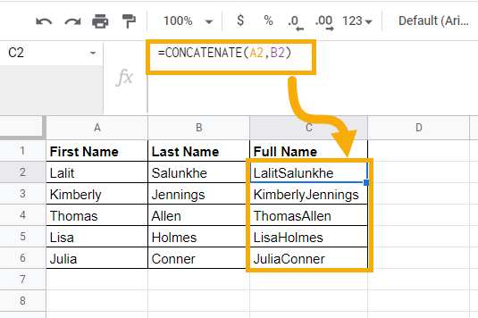
= CONCATENATE ( A2, B2 )

Insert the above formula into cell C2 to use the CONCATENATE function to join the first and last names together.

Since the first name is in column A and the last name in B, use the cell references A2 and B2 respectively as string1 and string2 arguments inside the CONCATENATE function. You need to separate these arguments using the comma.

You can drag this formula across the remaining rows or copy and paste it down those rows as well.

The final output will be as shown above.

= CONCATENATE ( A2, " ", B2 )

You might have noticed that the first and last names have no space between them. You can use any other delimiter between them. Just make sure to add it inside the formula.

The formula above returns the first and last name with space between them.

Make sure you encase the space character in double quotes within the formula. Also, note to yourself that the space here is a string argument and combined with the first and last name.

The advantage of using the CONCATENATE function is that you can use multiple strings as arguments inside it and get them appended to one another. You can use a different delimiter for each string as well. Such a versatile function, isn’t it?

Note: You can only use a maximum of 253 arguments to combine together inside the CONCATENATE function. But you’ll be unlikely to ever hit this limit.

Combine First and Last Name Using the TEXTJOIN Function

Another function made for combining text is the TEXTJOIN function.

The function takes two or more text values as an argument and allows you to combine them based on a specific delimiter.

The benefit of using this function over previously discussed ones is that it allows you to ignore any blank cells in your data.

Syntax for the TEXTJOIN Function

TEXTJOIN ( delimiter, ignore_empty, text1, [text2, …] )

• delimiter – This is a mandatory argument that specifies the delimiter based on which you ask the system to separate the text after concatenation happens. Most of the time, users prefer to use the white space as a delimiter. However, you are free to use any other special characters such as a comma, a hyphen, forward slash, or for that matter, a dollar, a pound sign as well. Make sure you enclose the value for this argument inside double or single quotes.
• ignore_empty – It is also a mandatory argument that takes two logical inputs, TRUE or FALSE, to specify whether the formula should ignore the empty cells or not. If provided with TRUE, the formula will ignore the empty cells or values from the calculation.
• text1 – a required argument. Specifies a string or a range of cells containing strings. You at least should provide one text value or cell/range containing text values for this formula to work.
• [text2, …] – a secondary argument that is optional. It also specifies a string or a range of cells containing strings.

Combine First and Last Name Example

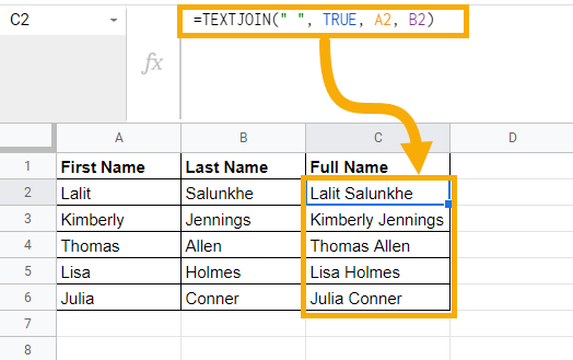
= TEXTJOIN (" ", TRUE, A2, B2 )

Insert the above formula into cell C2 to combine the names together with the TEXTJOIN function.

The first argument is to specify the delimiter based on which you want to separate the text after the concatenation happens. You can use any delimiter of your choice. However, the most suitable choice is to use the space character in this case.

The second argument gives you the liberty to ignore the blank cells. If you type TRUE, the formula will ignore any blank cells. If FALSE is used, the blank cells will be kept. It would be best if you use TRUE as a value for this argument in case there are any missing names.

The first name is in cell A2, so use it as an input value for the text1 argument.

Even though the second argument is optional, you have the last name inside cell B2, and you should use it as a second text argument.

You can drag the formula down until cell C6 to expand this formula for all cells where first name and last name exist.

The final output is as shown in the screenshot above.

=TEXTJOIN("-", TRUE, A2, B2)

Pro Tip: You can experiment with different special characters as a delimiter while concatenating first and last names using the TEXTJOIN function. One illustration is as shown above, where a hyphen is used as a delimiter. The formula that does this task is as shown above.

= TEXTJOIN ( " ", TRUE, A2:B2 )

There is an even better way of joining adjacent cells with the TEXTJOIN function. You can reference a single range in the last argument and it will join each cell in the range.

In the above formula, you only need to reference the range A2:B2 to join the first name and last name in A2 and B2.

The advantage of using this function over all others is that you have the delimiter argument as a parameter. You don’t need to specify it repeatedly as you do inside the CONCATENATE function or while using the ampersand operator.

The function also has its own way of dealing with blank cells. You can specify whether you want it to ignore the blank cells or keep those within the results.

Note: Keep in mind that the function only allows 252 text arguments, and anything above that will parse an error within this formula. Moreover, the resulting string length should also be lesser than or equal to the cell limit of 32,767 characters. Anything above that will also cause errors.

Combine First and Last Name Using the Smart Fill Option

Ever since its introduction in Google Sheets, Smart Fill has become extremely popular among users.

It’s a power-packed AI feature that recognizes patterns, and can generate corresponding formulae, and applies those automatically throughout the column.

This feature brings revolution into the world of data entry as the AI-powered tool learns the patterns by which you type the data, then it suggests a better way to do it by either providing formula or by autocompleting the remaining cells.

Check out this post that will show you everything you need to know about Smart Fill for further details on this amazing feature.

To combine the first and last names using Smart Fill, follow the steps below.

• In cell C2, type the first name and last name together as you want. I will type out Lalit Salunkhe.
• In cell C3 as well type the same way. The second name will be Kimberly Jennings.

These two entries should be enough for Google Sheets to recognize the pattern.

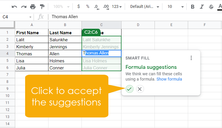
In cell C4, when you start typing the name, you will see that the Smart Fill pop-up will appear suggesting that this operation can be done based on a formula.

The AI engine that powers the autocomplete feature recognizes the pattern based on which columns A and B’s arguments are combined together. It then suggests a formula that can work on this task and get it done.

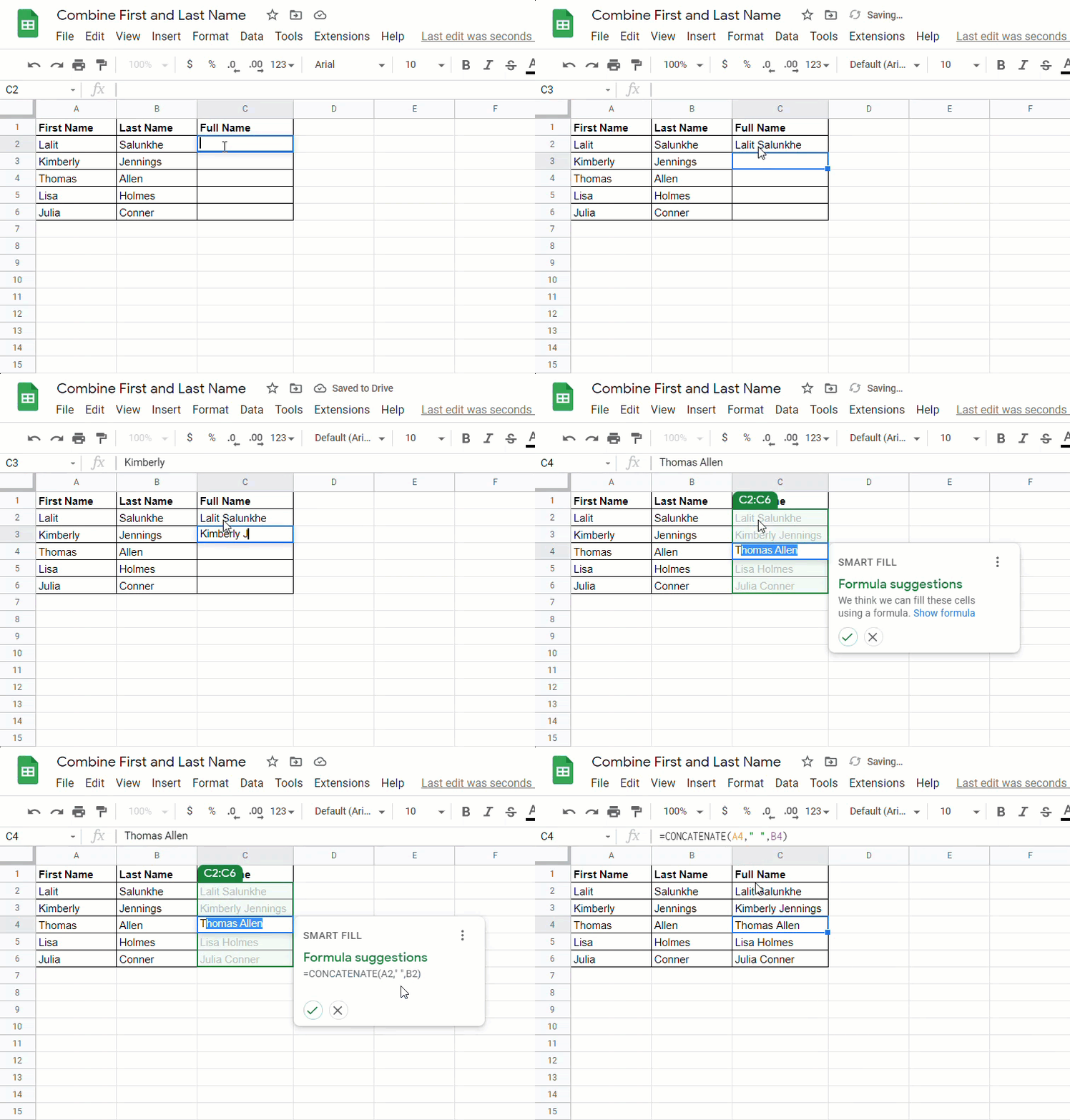
You can then click on the checkbox to accept the suggestions provided.

As soon as you check it, the remaining cells will be populated automatically with the first and last names combined as you were expecting.

The best part about using this method is that Google Sheets and its AI engine recognize the pattern while typing the first two full names.

It then searches for a ways which it can do this task. Finally, it suggests the formula that does this.

If there is no formulated way available, it will auto-fill the text based on the pattern learned. This approach reduces errors that might occur if this was a pure data entry task.

There is a possibility that the Smart Fill feature is not working at all for you in the Google Sheets environment. For such instances, you need to enable it manually to work.

Follow these steps to enable the Smart Fill feature.

Inside Google Sheets, go to the Tools menu and click on it to expand available options.

Select the Autocomplete option. It will have three options in the submenu.

• Autocomplete the text based on a recognized pattern.
• Suggest a formula to do the task.
• Autocorrect the formulas, respectively.

You can enable ones that are of your interest. However, I would recommend enabling all the options as they are really very helpful.

Note: There is a shortcut to do this task. You can use the Ctrl + Shift + Y key combination to check if any Smart Fill tools can be used on the given range of data or not.

Combine First and Last Name Using the Apps Script

If you are someone who likes to automate things rather than typing formulae and setting ranges manually, the Google Apps Script environment is for you.

The JavaScript-based cloud platform will allow you to write code that can automate simple or complex tasks in your day-to-day Google Workspace life.

If you are new to Apps Scripts, you should definitely read our article that will turn you into an Apps Script pro! It will be worth the time to learn how you can automate tasks inside the Google Workspace.

You can write a script inside the Apps Script that combines first and last names with a specified delimiter.

Firstly, open the Apps Script environment. You can do it by navigating towards the Extensions menu and click on the Apps Script to launch it in a new tab.

After you launch the tool, copy and paste the following code inside the script environment. We will discuss the script and its working step by step.

function ConCat() {
    var sheet = SpreadsheetApp.getActiveSpreadsheet().getSheetByName("Data");
    var lastRow = sheet.getLastRow();
    //Get values from the First Name column
    var firstName = sheet.getRange(2, 1, lastRow,1).getValues();  
    //Get values from the Last Name column
    var lastName = sheet.getRange(2, 2, lastRow,1).getValues();  
    //Create an empty array that can hold the concatenated values
    var fullName = [];

    //Add items to the fullName array
    for(var i=0; i<lastRow; i++){
        fullName[i] = [firstName[i][0]+" "+lastName[i][0]]
    }

    //Post the result back to Full Name column (column C) starting from row 2
    sheet.getRange(2, 3, lastRow, 1).setValues(fullName);
}

1. On the first line, you define a function that can hold the entire code you are going to write. You name it as conCat(). You can name it anything of your choice though.
2. Then, you define a sheet variable that takes a worksheet named Data from the active spreadsheet. You then use the SpreadsheetApp.getActiveSpreadsheet().getSheetByName() method to get the sheet by name.
3. To get the last active row inside this sheet, you have to use the getLastRow() method called on the sheet variable. The results are then stored in the lastRow variable.
4. Inside the firstName variable, this takes values from column A starting from the second row. You have to use the sheet.getRange().getValues() method to get this done. The getRange() method takes data starting from the second row in the first column, generating a one-dimensional array from the second row until the last working row, and finally taking all the values from that array.
5. Similarly, the lastName variable stores all the values from column B, starting from the second row until the last working row.
6. In the next line of code, you have to create an empty array that can store the concatenated result within it. Name it as fullName.
7. After defining an empty array that could store the results, the next task is to populate values to that array. You are going to use the for loop in this task. The for loop runs for each row starting from 0 until the last working row. For each row, first name and last names are combined together with space as a delimiter and stored into the respective row position inside the fullName array.
8. Finally, you have to use the getRange().setValue() method to populate these values to column C inside the same sheet. The getRange() method creates a one-dimensional array starting from the second row in the third column until the last working row. The setValue() method then populates the result from the fullName array to this column.

To run the code above, click on the Run button from the Apps Script menu and see the output generated that automatically combines the first and last names, then populates the combined output to column C.

Conclusion

There are lots of ways of combining text inside google sheets.

Using the ampersand operator to combine first and last name is easy when you have only two arguments to combine.

The CONCAT function is explicitly designed to combine exactly two text values, but lacks any way to delimit the results with a space.

The CONCATENATE function is the best way of combining two or more strings together.

The TEXTJOIN function allows you to specify delimiter as an argument. You don’t have to specify it again and again like the CONCATENATE function or the ampersand operator. This one also allows you to reference a single range of values to join.

The Smart Fill option is revolutionary and provides AI-powered ways of auto-filling the cells by recognizing user patterns, suggesting formulas to get work done, and autocorrecting the formulas whenever possible.

Apps Script way of combining first and last names is for those who want to write a small piece of code to automate this task instead of using the functions and providing arguments.

Do you use any of these great techniques for merging text values? Do you know any other methods I missed? Let me know in the comments below!